Position Identification

Monitoring is not supported by Everest (EVE) drives through CANopen communications. Therefore, in order to carry out Mechanical Tuning please connect to the drive via Ethernet. The feature is supported on EVS.

Introduction

This "Position Identification" is the first step to configure and tune the PID controllers for the position loop of the drive. The main goal is to identify a model which it will be different depending on if your system has a gear or an ideal integrator.

In this document you will see an overview about the two types of identification and also how to use them. Also, the information that charts provide.

Types of identifications

There are two types of identifications:

• Theoretical identification (green)

• Automatic identification (orange)

The controller can be designed from the theoretical parameters as provided in the datasheet of the motor.

The drive is able to identity the plant on its own. We recommend this option as it provides a more realistic representation of the plant.

Charts

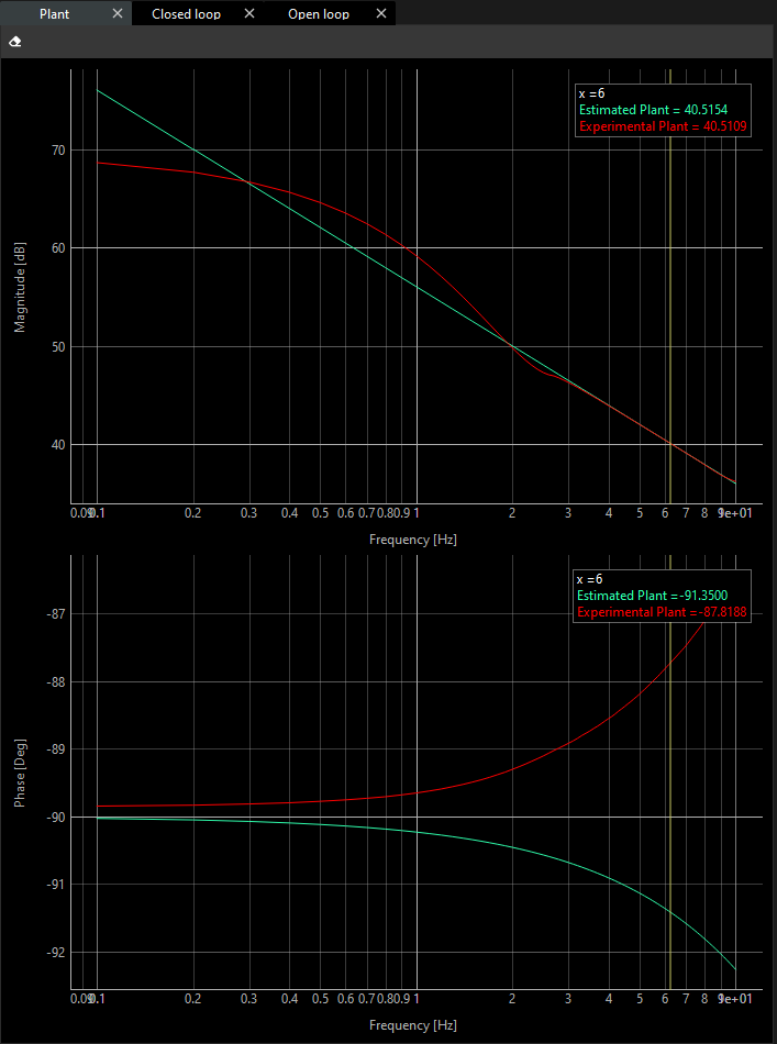
Both types of identifications show signals on the scope on the Plant tab.

The chart above shows the gain meanwhile the below shows phase in frequency domain.

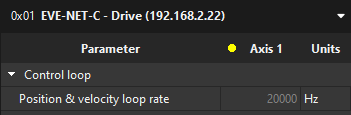
Display widget

If you want to see how loop rates are, you can see this information on the Display widget.

Theoretical identification

If you decide to make an automatic identification, you can skip the Theoretical Identification.

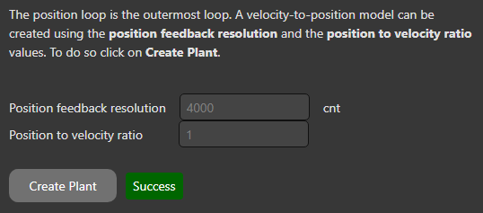
1. You will see the position feedback resolution and the velocity ratio parameters are the same values that you put previously at Feedbacks page. If you think you need to change them, go back to this page.

2. Click on the “Create Plant”.

3. Make sure that the test is passed successfully.

   

4. If the plant is created successfully, the theoretical plots in the magnitude and phase charts in the frequency domain are presented based on the type of model (ideal integration or gear), feedback resolution and friction.

   

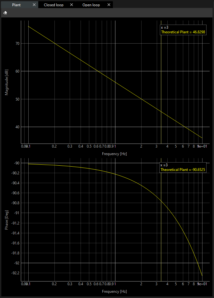
5. In addition, you will notice the Terminal shows the transfer function that plots comes from.

   

Automatic identification (recommended)

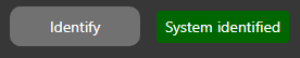
1. In order to do an automatic identification, click on the Identify button.

2. The result of the identification will be presented next to the Identify button. If it is successful, you can successfully continue the tuning. If it fails, recommendations for a better identification will be given in the terminal.

   

3. Then, you can notice two plots in each chart are printed. For a further clarification about these plots:

   1. The green one is an estimated plant, and it is given by a transfer function calculation.

   2. The red one is the response of the actual system.

   

4. In the terminal window, you can find the following information:

   • The quality of the identification.

   • The Transfer Function.

   • The type of the model (ideal integrator or gear).

5. You have successfully created the plant of your system.

6. Some very specific applications, might require changing the excitation parameters. This can be done through the Advanced Options.

   

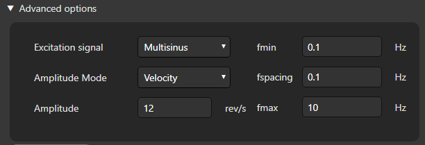
7. Here, you can set additional configuration:

   • Excitation signal:

     • Multisinus

     • Sinesweep

     • Chirp

   • Amplitude Mode: Just you can choose Velocity mode.

   • Amplitude: The Amplitude of the excitation signal in rev/s.

   • fmin: The minimum frequency used for the identification.

   • fspacing: The resolution of the frequency.

   • fmax: The maximum frequency.

8. When you decide your plant is correct, you can go to the next step.