Velocity Identification

Monitoring is not supported by Everest (EVE) drives through CANopen communications. Therefore, in order to carry out Mechanical Tuning please connect to the drive via Ethernet. The feature is supported on EVS.

Introduction

The "Velocity Identification" is the first step to configure and tune the PID controllers for the velocity loop of the drive. The main goal is to identify the JB model (inertia-friction) of the motor connected.

In this document you will see an overview of the two types of identification and how to use them. Also, it provides explanation on what the charts present.

Types of identifications

There are two types of identifications:

• Theoretical identification (green)

• Automatic identification (orange)

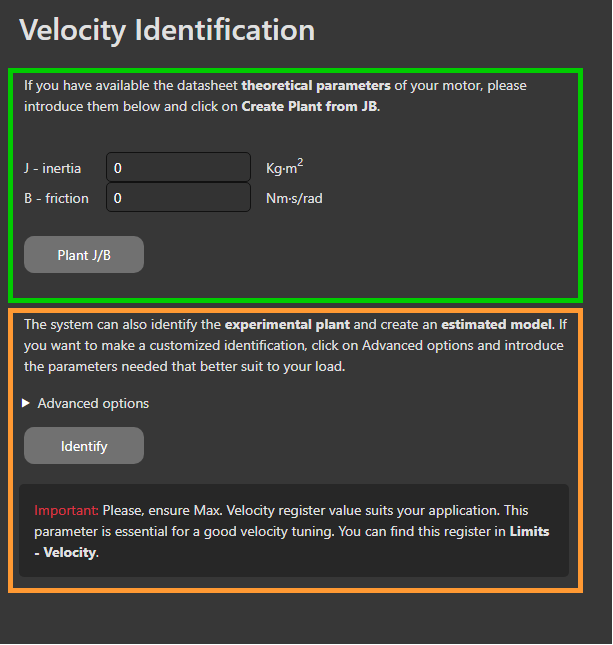
The controller can be designed from the theoretical parameters as provided in the datasheet of the motor.

The drive is able to identity the plant on its own. We recommend this option as it provides a more realistic representation of the plant.

Charts

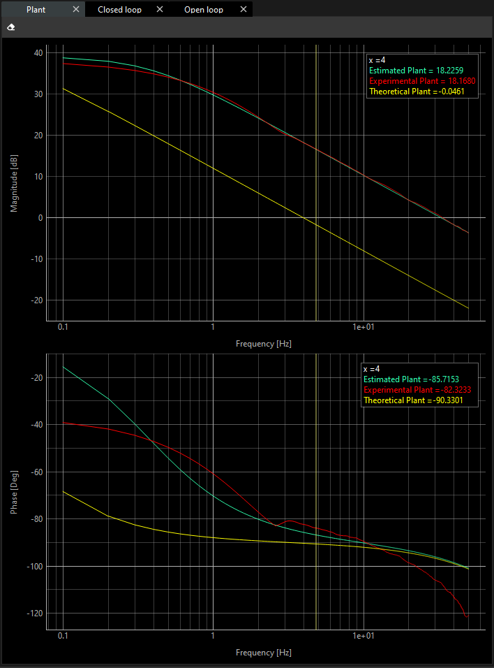
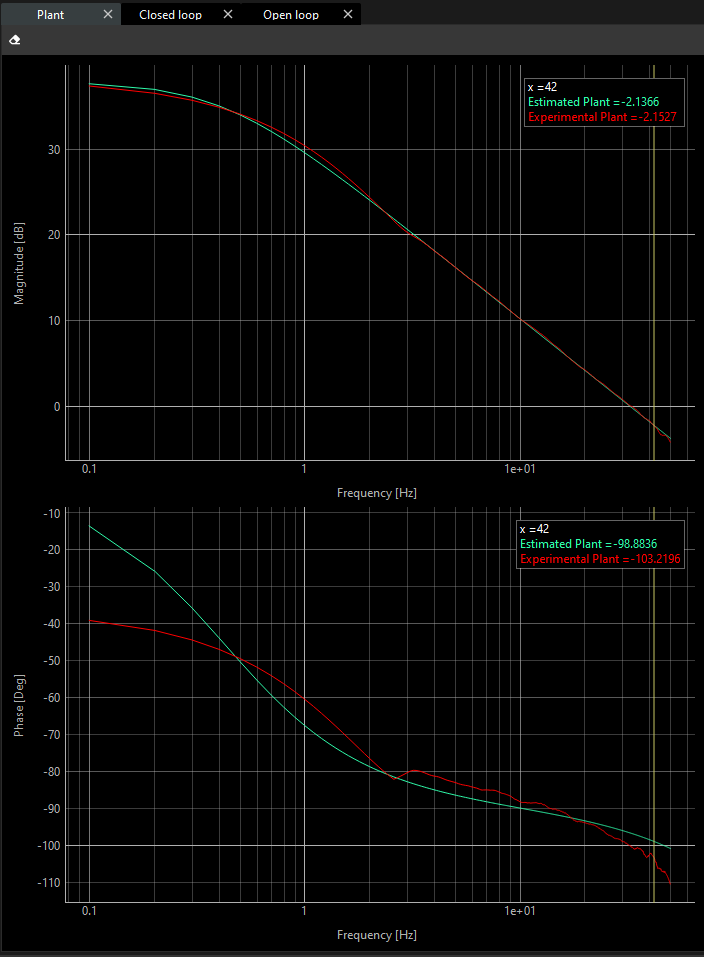
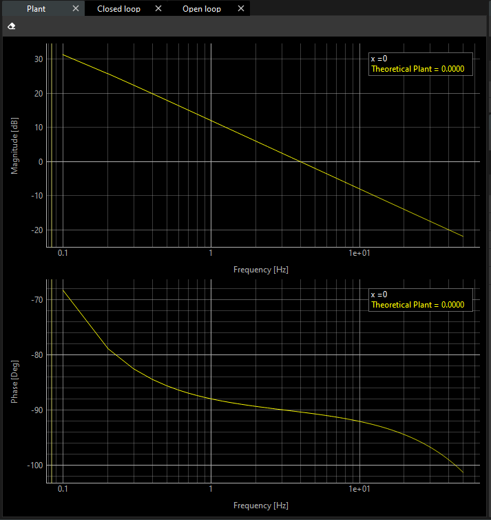
Both types of identifications will show some signals on the scope on the Plant tab

The chart above shows the gain meanwhile the below shows phase in frequency domain.

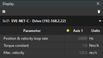
Display widget

If you want to see what the loop rates are, you can find this information on the Display widget. You can find more information in this document.

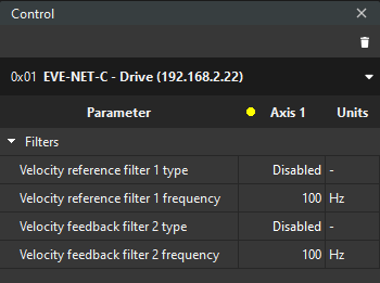
Control widget

If you consider you need to include a reference filter or a feedback filter, you can set up on the Control widget. You can find further information about these parameters at Filters and offset section.

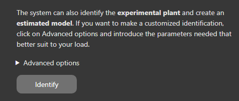
Automatic identification (recommended)

1. In order to do an automatic identification, click on the Identify button.

   

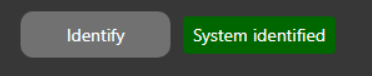
2. The result of the identification will be presented next to the Identify button. If it is successful, you can successfully continue the tuning. If it fails, recommendations for a better identification will be given in the terminal

   

3. Then, you can notice two plots in each chart are printed. For a further clarification about these plots:

   1. The green one is an estimated plant, and it is given by a transfer function calculation. This transfer function is calculated through inertia and friction estimated.

   2. The red one is the response of the actual system.

   

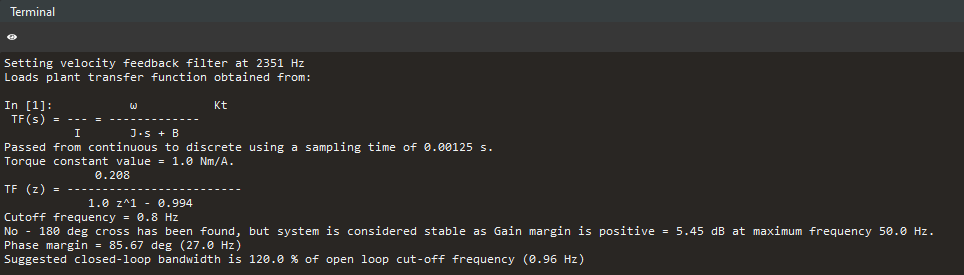
4. At terminal, you can find relevant information. For example:

   • The quality of the identification (correlation factor).

   • The Transfer Function.

   • Phase and Gain Margins.

5. You have successfully created the plant of your system.

6. Some very specific applications, might require changing the excitation parameters. This can be done through the Advanced Options.

   

7. You will have a dropdown menu

   

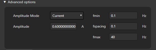
   Here, you can set additional parameters:

   • Amplitude: The Amplitude of the excitation signal in Amperes.

   • fmin: The minimum frequency used for the identification.

   • fspacing: The resolution of the frequency.

   • fmax: The maximum frequency.

8. When you decide your plant is correct, you can go to the next step.

Theoretical identification

If you decide to make an automatic identification, you can skip the Theoretical Identification.

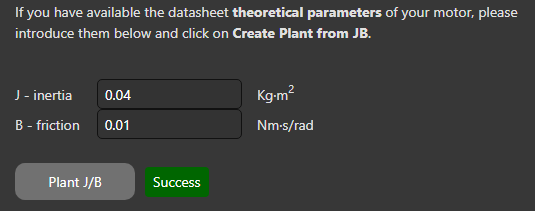
1. Put the inertia and friction, as presented in the datasheet of the motor.

2. Click on the “Plant J/B”.

3. Make sure that the test is passed successfully.

   

4. If the plant is created successfully, the theoretical plots in the magnitude and phase charts in the frequency domain are presented based on the theoretical inertia and friction.

   

5. In addition, you will notice the Terminal shows some information. This information includes:

   1. The transfer function that plots comes from.

   2. Some additional information about Gain and Phase margins.