Electrical Tuning: Frequency Design

Introduction

After having a proper identification of the system plant, you can configure the control loop.

You have to perform minimum one plant model in the previous step. Otherwise, this step will be disabled.

This page is not available if trapezoidal commutation is selected.

For further technical information about how Current control loop works, click on here.

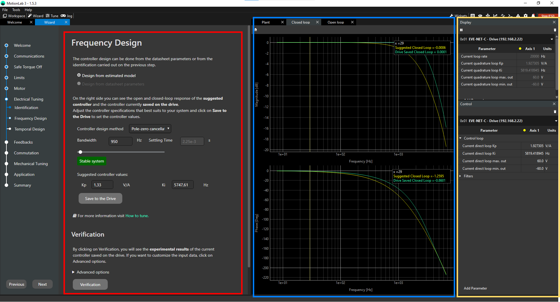
Overview of this page

There are 3 parts in this page:

System configuration and verification (red).
Bode diagrams of magnitude and phase (blue).
Display and Control widgets (yellow).

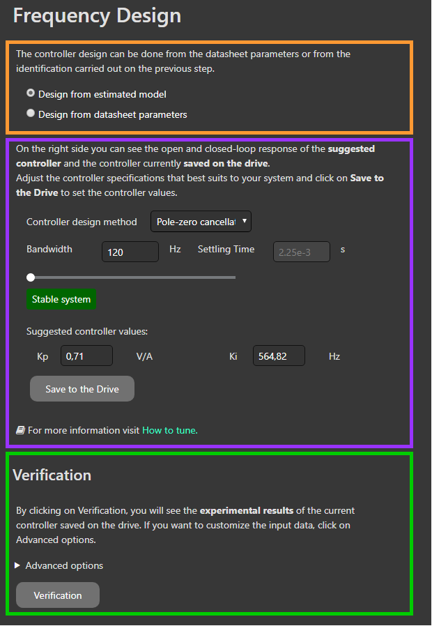
System Configuration and Verification

There are 3 main subparts:

Plant model choice (orange).
Control Loop configuration (purple).
System verification (green).

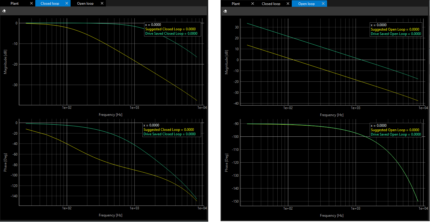
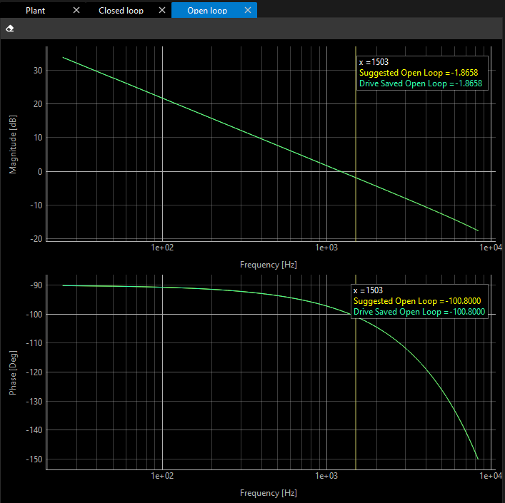
Bode diagrams of magnitude and phase

You have two tabs:

Closed loop (recommended)
Open loop

Both tabs show the Gain and Phase in frequency domain.

The Closed Loop Transfer Function (CLTF) is the most common way to describe the control system in the frequency domain. The data is taken while the loop is closed, so all of the closed loop dynamics are captured in this transfer function. The gain of the CLTF is very close to unity at low frequency and rolls off at high frequency, with some amplification in between. The phase of the CLTF is near 0 at low frequency and near -180 degrees at high frequency. This curve is typically used to state the system’s “Bandwidth”.

The Open Loop, or “Loop” transfer function (OLTF) is representative of all the frequency dependent blocks that make up of the servo loop, meaning the control, the drive, the plant, and the sensor. The OLTF for some systems can be taken with the servo loop open, but in many cases it must be either derived from the Closed Loop.

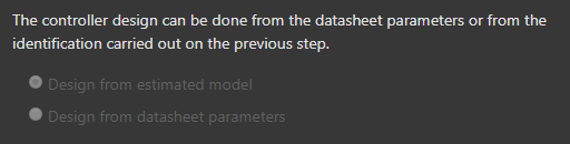
Plant model choice

Depending on the identification method used on previous page, Electrical tuning: identification, you should select the model you want to use to design your controller.

If theoretical identification was used, the only option will be “design from datasheet”.
If experimental identification was used, the only option will be “design from estimated model”.
If both were used, both options will appear.

Loop adjustment

The main goal of this step is to adjust the loop parameters: K_p and K_i. You can get them and simulate their implications for the system without saving in the drive. You will be able to see these simulations in different plots.

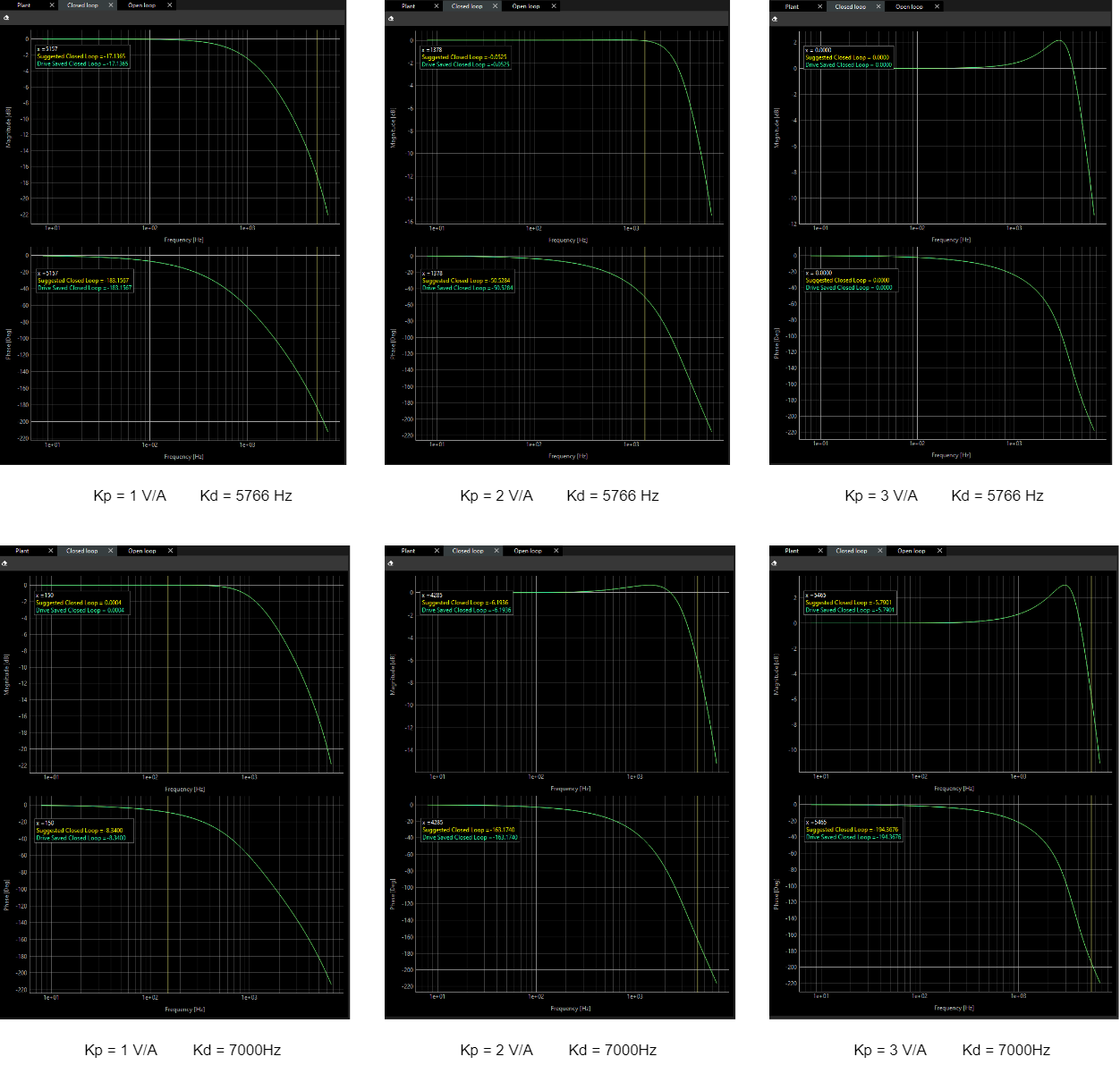
Once you consider these parameters works properly, you can save them into the drive. You can see below several examples about how the closed loop behaves with different K_p's and K_i's.

Methods

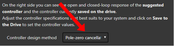
In order to do that you have to choose which methodology you want to apply.

There are 3 possible methods:

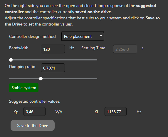
Pole placement: You will be able to tune the system response quickness and overshoot with Bandwidth and Damping ration.
Pole-zero cancelation: You will be be able to choose the system response quickness for a stable system (where the zero is cancelled)
Manual: You will be able to chose Kp and Ki freely.

Pole-zero cancellation and Pole-placement are automatic methods that calculate the K_p an K_i. Manual is to adjust the parameters manually and see the frequential response.

For more information about these parameters, go to the How to Tune page.

Pole placement

Pole-zero cancelation

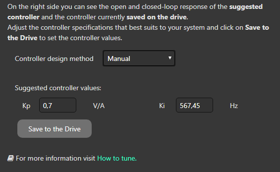
Manual

Example

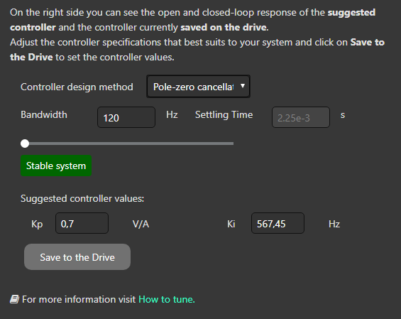
In the case of Pole-zero cancellation.

If you move the Bandwidth slider or directly you edit the its value directly, K_p and K_i parameters will be modified automatically.

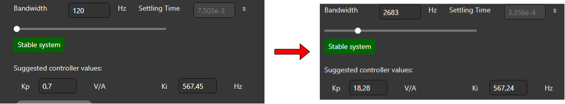
The label under the slider indicates the stability of the system

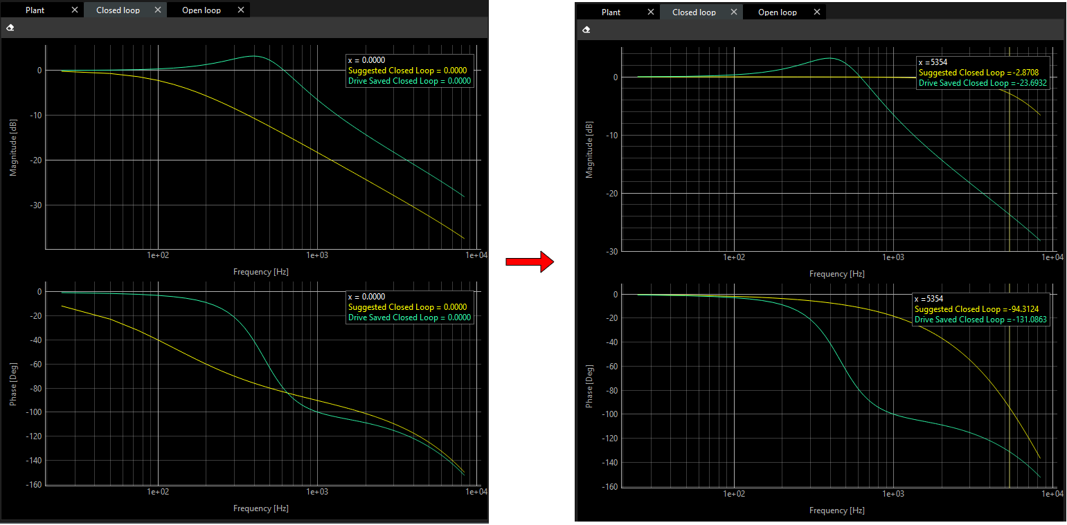
Check the frequential response of your system and adjust the slider until the expected result is obtained. Also, you can compare the response of the controller values saved on the drive against the suggested new ones.

For more information, go to the How to Tune page.

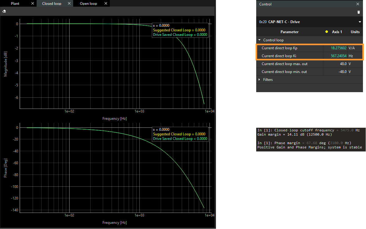
You have further information as well in the Terminal:

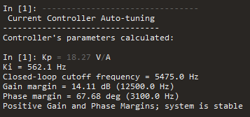
However, these loop parameters will not be set into your drive automatically. You have to click on the button “Save to the Drive”.

In order to check if they are properly saved, you can see:

These parameters in the Control widget in green color.
Drive Saved Closed Loop plots change their shape like Suggested Closed Loop.

Verification

To compute it, just click on the “Verification” button.

In this step, the main goal is checking how your actual system works with the current controller saved on the drive.

Let’s continue the example before.

Example

In order to make a verification, you can follow the steps below:

Modify the bandwidth value.
Click on the “Save to the Drive” button.
And click on the “Verification” button.

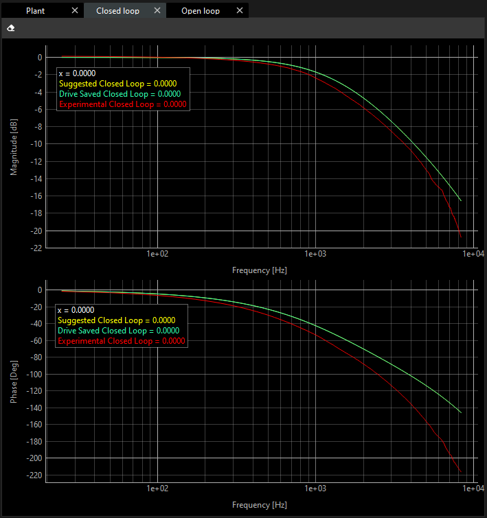
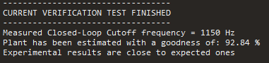
Finally we get a message below that tells us.

Charts are updated as well.

The terminal shows the quality (goodness) of the verification. This goodness compares the simulate results with the experimental ones.

Some very specific applications might require changing the excitation parameters. This can be done through the Advanced Options.

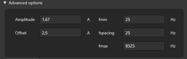
These options are the same as you configured previously at identification step. In fact, that values are linked, and the same identification used in identification is used at verification.

These parameters are:

Mode: In verification no mode can be selected, since the excitation on the current loop is always in current. See Section Automatic identification - Step 8 for further details.
Amplitude: The maximum current amplitude.
Offset: How many units increase or decrease the continue with respect to the zero level.
fmin: The minimum frequency that the plant is made.
fspacing: The resolution of the frequency.
fmax: The maximum frequency.

The simulation results are represented in closed-loop and open-loop.

In these charts there are no Experimental Closed Loop plots, just the estimated ones.

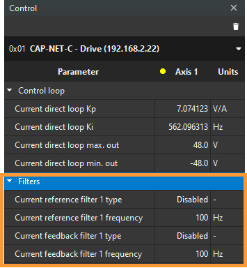
You can use two filters per signal for your system:

Two for the current reference
Two for the current feedback

You can enable/disable at Control widget.

You can find further information at Filters and Offset section.