Set-point manager and interpolation buffer
These modules allow generating different profiles and managing burst of set-points for applications where the main device/instance cannot be fast enough and deterministic for generating its own profiles.
On one hand, the set-point manager is in charge of:
Enabling and configuring the available profiles.
Generating a profile point on each control loop cycle.
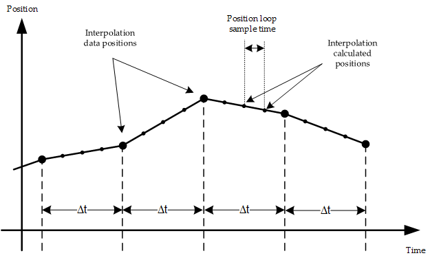
Additionally, the interpolation buffer allows storing set-points to be injected into the profiler later. When enabled, the set-point manager takes a new input from the interpolation buffer at a given rate and injects it into the active profile. The rate at which the set-points are extracted from the buffer can be determined by 0x21F0 - Interpolation time exponentand the 0x21EF - Interpolation time mantissa or by the introduced duration if the PVT operation mode is selected. The profile output is directly connected to the demand of the chosen mode of operation (Position, Velocity or Current).
The profiles are not available on every selected mode of operation. For example, profiles cannot be connected to any voltage mode. Further details about what is available on each mode are:
Current modes (CSC, C, CA)
Velocity modes (CSV, PV, V)
Position modes (CSP, PP, IP, P)
Modes using only profiles are referenced in this documentation as profile mode. Modes combining profile and the interpolation buffer are called in this documentation interpolated modes.
Profiles
Linear profile
This mode is time-restricted and interpolation time exponent and interpolation time mantissa are inputs of each movement. The output is a linear trajectory linking the start and end points. The desired interpolation time determines how far apart the start and end points are located and the slope of the linear trajectory.
Note
The profile will start generating points depending on the selected profiler latching mode. If latching is disabled, the linear profile starts immediately upon a change of the set-point. If latching is enabled, the linear profile starts after a change of set-point, and its confirmation through new set-point bit from the control word.
Whenever this mode is not used in combination with the interpolation buffer, the time for each movement is defined by Interpolation time mantissa * interpolation time exponent. If the interpolation buffer is used, the interpolation time may be provided by the buffer itself. See more details below.
Note
If the resulting interpolation time is smaller than the update time of the system, an error will be reported.
Trapezoidal profile
This mode follows an online trapezoidal profile with 3 stages:
Linear acceleration stage
Constant velocity stage
Linear deceleration stage
In some cases, if the profile step is too small, the requested constant velocity stage is not reachable. The movement gets done in two stages:
Linear acceleration stage
Linear deceleration stage
This profile is defined by three parameters:
If this profile is enabled for velocity modes, the profile is composed of 2 stages:
Linear acceleration / deceleration stage
Constant velocity (velocity set-point or Max. velocity)
The third stage is not executed.
This profile is not time-restricted.
Note
The profile will start generating points depending on the selected profiler latching mode. If latching is disabled, the linear profile starts immediately upon a change of the set-point. If latching is enabled, the linear profile starts after a change of set-point and its confirmation through new set-point bit from the control word.
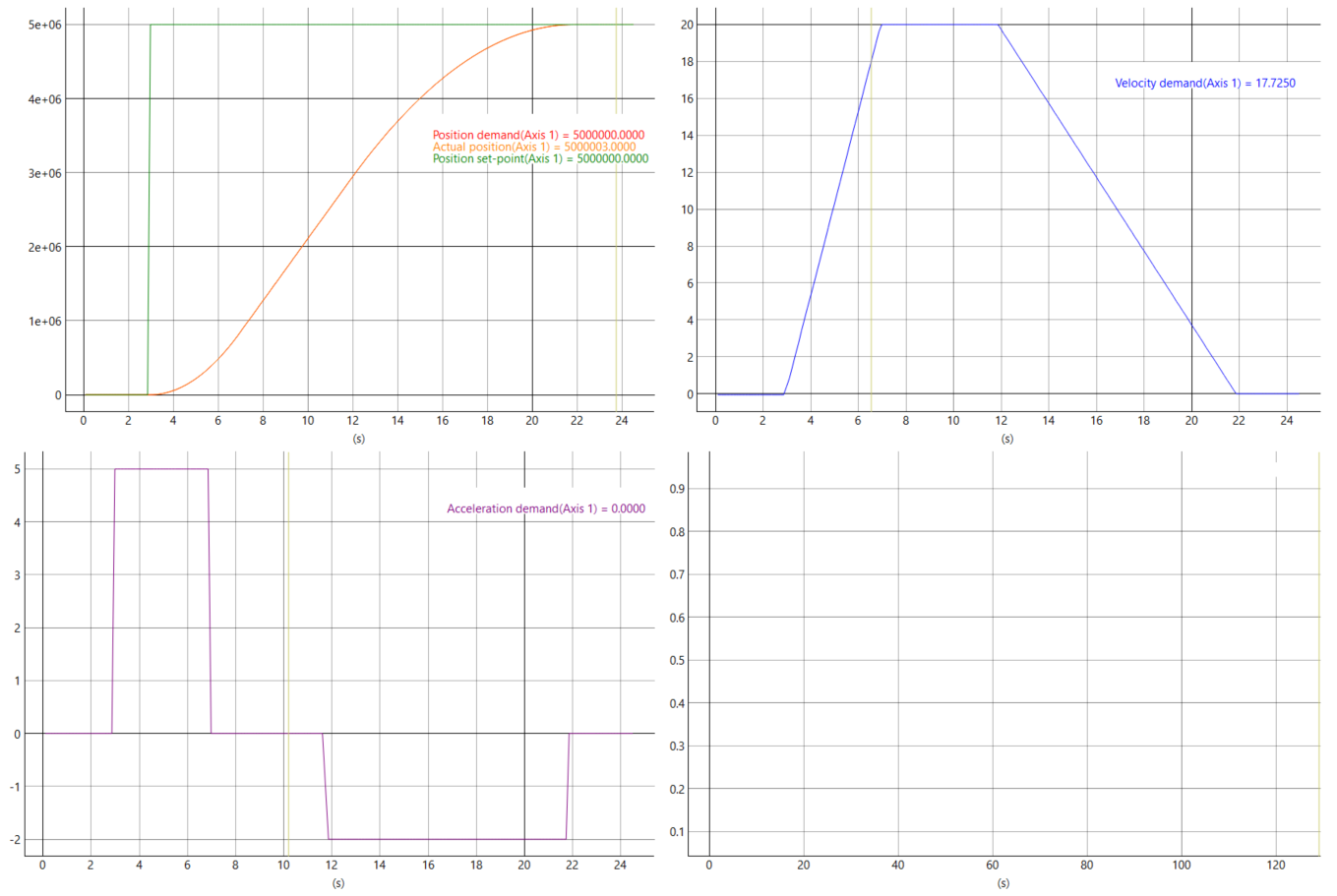
The following picture shows a trapezoidal velocity trajectory in a profile position (PP) movement.
S-curve profile
This mode internally generates an offline trapezoidal profile and joins the resulting transition points of the trapezoid with 5th-degree polynomials to soften the trajectories at each stage. These polynomials are described at the end of this document.
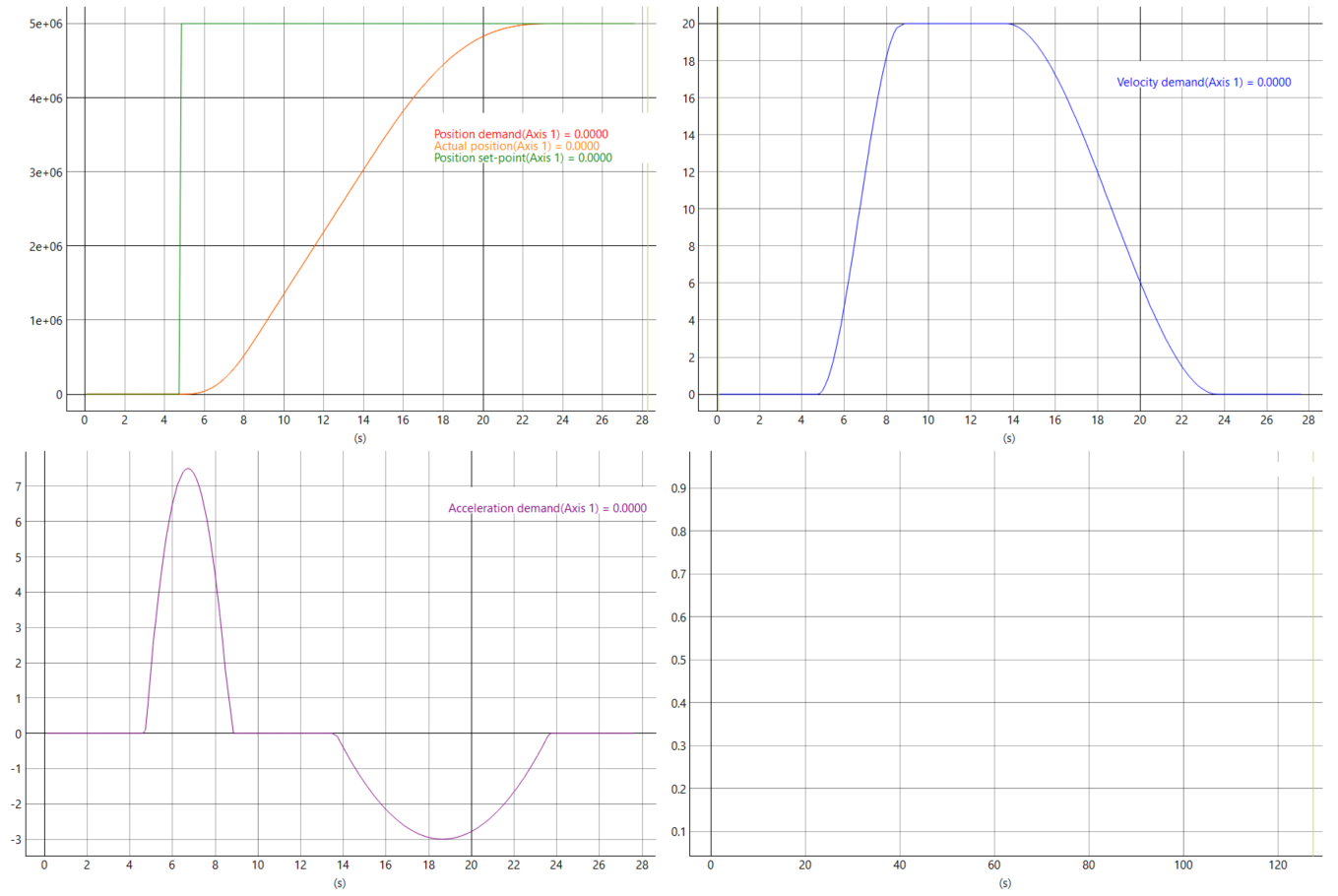
The following picture shows an equivalent movement of the example above, but using a S-curve velocity trajectory in a S-curve profile position (SPP) movement.
Note
Note that the resulting polynomial curves will require a higher acceleration than the trapezoidal acceleration and decelerations for a fixed trajectory time.
PVT profile
This mode joins a start and endpoint with a 5th-degree polynomial trajectory, and can only be used in combination with the interpolation buffer. The information to generate the profile are initial position, velocity, acceleration and time, and final position, velocity, acceleration and time. These are fed internally by the interpolation buffer once the user has introduced a list of final positions, velocities, and movement durations.
More information about these polynomials can be found at the end of this document.
Note
All movements in this mode assume acceleration is 0 at the beginning and end of each movement.
Warning
The generated PVT profile does not take into account the limits of the motor to generate its trajectories. This means that the main device/instance should take care of ensuring that the requested trajectories can be physically performed within the average limitations of the motor.
Interpolation buffer
The interpolation buffer is a buffer of set-points Depending on the operation mode active, the buffer will hold the position, velocity, and time duration set-points. In combination with the linear and 5th-degree polynomial profiles, it extends the profile generation capabilities for main devices/instances that are neither fast nor deterministic enough to generate each point of a complex profile at the right time. The idea is to fill a set of position set-points in the buffer through a network burst and then let the drive inject the stored set-points into the set-point manager, while the main device/instance computes the next set of targets and refills the interpolator buffer.
x20c4
If the interpolator buffer is combined with the linear profile, the resulting mode of operation is called IP: interpolated position mode.
If interpolator buffer is combined with the 5th-degree polynomial profile, the resulting mode of operation is called PVT.
The related registers are the following:
0x2181 - Interpolation data record - Position input . (Mandatory) It contains the position to be stored in the buffer. It is required for the profiles:
Linear profile
5th-degree polynomial profile
0x2182 - Interpolation data record - Velocity input . (Optional) It contains the velocity to be stored in the buffer. It is required for the profiles:
5th-degree polynomial profile
0x2183 - Interpolation data record - Time input . (Optional) It contains the movement time to be stored in the buffer. It is required for the profiles:
5th-degree polynomial profile
0x2184- Interpolation data record - Integrity check (Mandatory) - Used to store the previous fields into the buffer. It is required for the profiles:
Linear profile
5th-degree polynomial profile
Procedure to fill a point in the interpolator buffer
Make sure that the 0x21F0 - Interpolation time exponent and the 0x21EF - Interpolation time mantissa are correctly configured.
Set the Operation mode to Interpolated Profile using the operation mode register 0x2014 - Operation mode.
Use the control word to enable the drive 0x6040 - Control Word.
Write the required input: ( 0x2181 - Interpolation data record - Position input / 0x2182 - Interpolation data record - Velocity input / 0x2183 - Interpolation data record - Time input)
Increment the integrity check value by 1 (0x2184- Interpolation data record - Integrity check) . When the drive detects an increment of 1 in the integrity check, it will save the configured values in the position, velocity, and time inputs.
Finally, start the movement through the run set-point manager bit from the control word, setting it to 1.
Note
If the selected operation mode is interpolated position mode, the Interpolation data record - Time input is not used and timing is replaced by the default interpolation time (given by the interpolation time mantissa and interpolation time exponent) of the drive.
The interpolation buffer works as a FIFO (First Input First Output). That means that new set-points can be added into the buffer while the set-point manager is extracting them. For proper management of the buffer, a set of parameters are available:
Interpolation buffer number of elements. Shows how many elements are inside the buffer.
Interpolation buffer maximum size. Shows the maximum buffer size allowed by the drive.
Interpolation data record status. Reports the status of the interpolation buffer.
On the other hand, if it is required to remove all the stored set-point from the interpolator buffer, the command interpolation data record force clear will clear the buffer allowing to add new set-points.
How 5th-degree polynomials work
5th-degree polynomials can be used to create time-dependent trajectories given some initial and final conditions. The 5th-degree polynomials are described by the following equation. This equation is used for position calculation, but its derivatives can be used for velocity, acceleration, and jerk.
When this polynomial is going to be used to describe a position trajectory, coefficients a0 to a5 can be calculated with the following expressions:
Where:
q0: Initial position
h: Total displacement
v0: Initial velocity
v1: Final velocity
acc0: Initial acceleration
acc1: Final acceleration
T: Movement time
Note
All movements in this mode assume acceleration is 0 at the beginning and end of each movement.
Although the jerk is not controlled and can be higher or lower depending on the movement's length and maximum acceleration, the acceleration is kept continuous and gradual.